Pneumonia Detection from chest radiograph (CXR)

Pneumonia accounts for over 15% of all deaths of children under 5 years old internationally. In 2015, 920,000 children under the age of 5 died from the disease. While common, accurately diagnosing pneumonia is difficult. It requires review of a chest radiograph (CXR) by highly trained specialists and confirmation through clinical history, vital signs and laboratory exams.

An example chest radiograph looks like this:

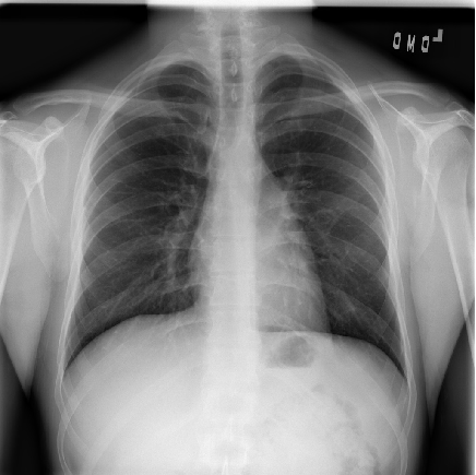
Pneumonia usually manifests as an area or areas of increased lung opacity on CXR.

However, the diagnosis of pneumonia on CXR is complicated because of a number of other conditions in the lungs such as fluid overload (pulmonary edema), bleeding, volume loss (atelectasis or collapse), lung cancer, or post-radiation or surgical changes. Outside of the lungs, fluid in the pleural space (pleural effusion) also appears as increased opacity on CXR. When available, comparison of CXRs of the patient taken at different time points and correlation with clinical symptoms and history are helpful in making the diagnosis.

In addition, clinicians are faced with reading high volumes of images every shift. Being tired or distracted clinicians can miss important details in image. Here automated image analysis tools can come to help. For example, one can use machine learning to automate initial detection (imaging screening) of potential pneumonia cases in order to prioritize and expedite their review. Hence, we decided to develop a model to detect pneumonia from chest radiographs.

Dataset

We used the dataset of RSNA Pneumonia Detection Challenge from kaggle. It is a dataset of chest X-Rays with annotations, which shows which part of lung has symptoms of pneumonia.

Chest Radiographs Basics

In the process of taking the image, an X-ray passes through the body and reaches a detector on the other side. Tissues with sparse material, such as lungs, which are full of air, do not absorb X-rays and appear black in the image. Dense tissues such as bones absorb X-rays and appear white in the image. In short -

• Black = Air
• White = Bone
• Grey = Tissue or Fluid

The left side of the subject is on the right side of the screen by convention. You can also see the small L at the top of the right corner. We see the lungs as black in a normal image, but they have different projections on them - mainly the rib cage bones, main airways, blood vessels and the heart.

Lung opacity

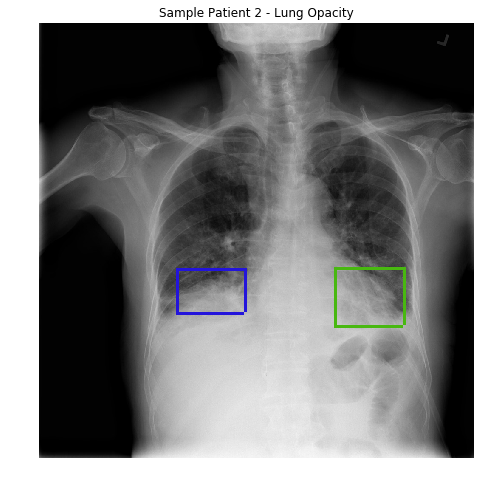
In loose terms, any area in the chest radiograph, that is whiter than it should be, can be considered as opacity. If you look at the above radiograph of Sample Patient 2, you can see that the lower boundary of the lungs is obscured by opacities. But in the previous image, you can see clear difference between the black lungs and the tissue below it, and in the image of Sample Patient 2 there is just this fuzziness.

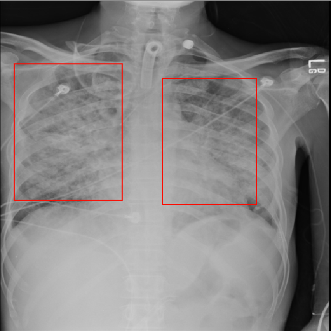
I will show you more images of normal lungs and lungs with opacity:

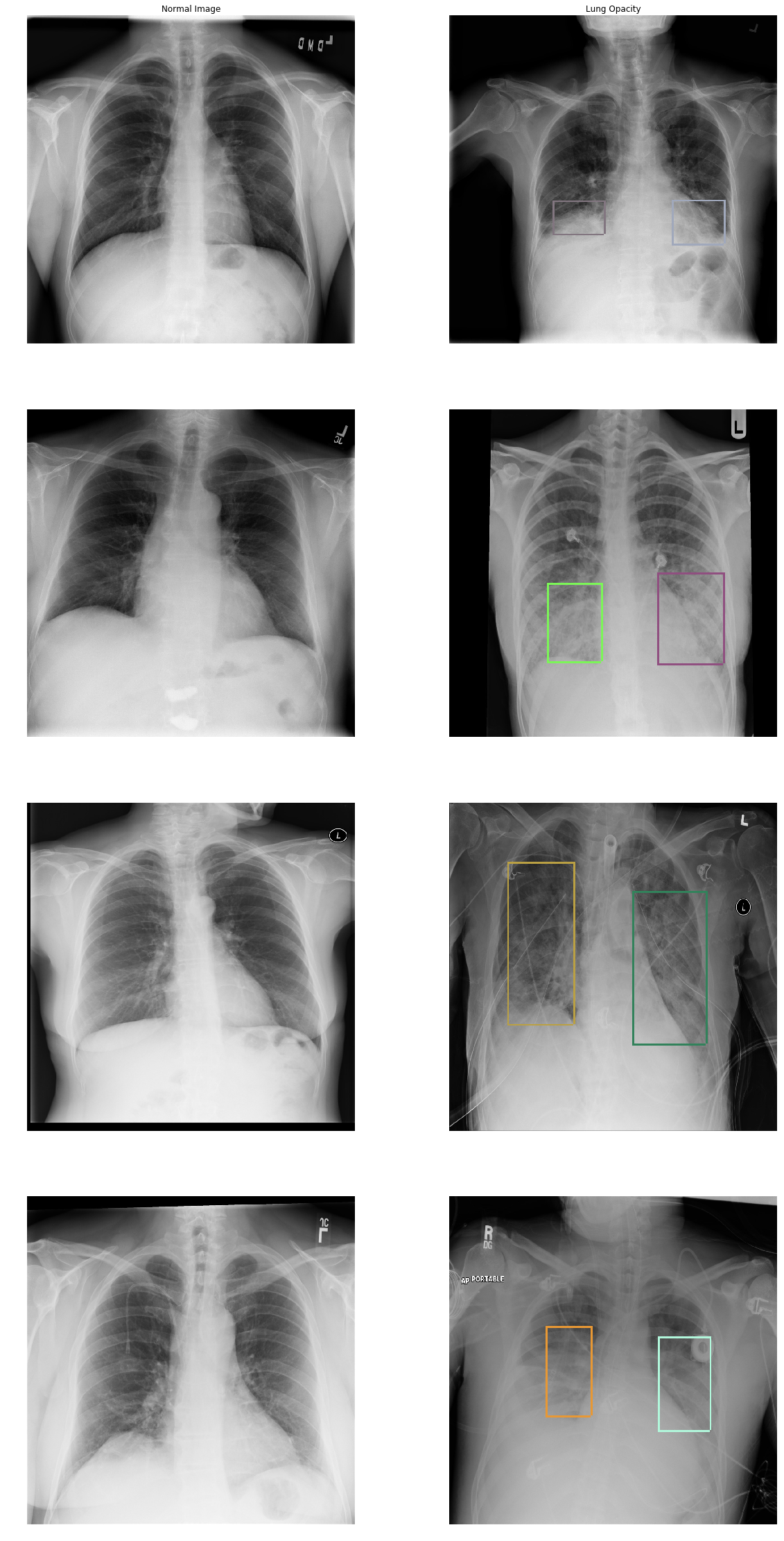
In the Lung Opacity images we can see that there is haziness were the labeled boxes are (termed ground glass opacity) and/or a loss of the usual boundaries of the lungs (termed consolidation). You can also see that patients with pneumonia are ill and have different cables, stickers, and tubes connected to them. If you see a round white small opacity in and around the lungs it’s probably an ECG sticker.

Install machine learning tools

We will use Intelec AI to train a model to detect pneumonia. You can download and install it for free from here.

Data preparation

We downloaded the training images (stage_2_train_images.zip) and annotations (stage_2_train_labels.csv) from kaggle. All provided images were in DICOM format. The annotations file looked like this:

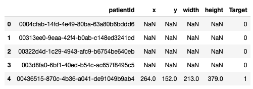
First row in the above image corresponds to patient with ID ‘0004cfab-14fd-4e49-80ba-63a80b6bddd6’. ‘Target’ column is 0 for this row. It means this patient doesn’t have pneumonia. On other hand, patient in the last row has pneumonia because of the area on the corresponding chest radiograph (xmin = 264, ymin = 152, width = 213, height = 379) with opacity.

We decided to use SSD object detector. It requires the annotation file to have columns image_name, xmin, ymin, xmax, ymax and class_name. Therefore we transformed our data into that format:

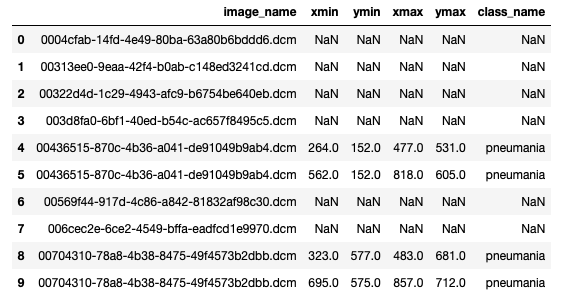
First 4 images in the above picture (lines 0 - 3) has no pneumonia annotations. On the other hand, image ‘00436515-870c-4b36-a041-de91049b9ab4.dcm’ has 2 annotations (lines 4 and 5). We saved it in “annotations.csv” file.

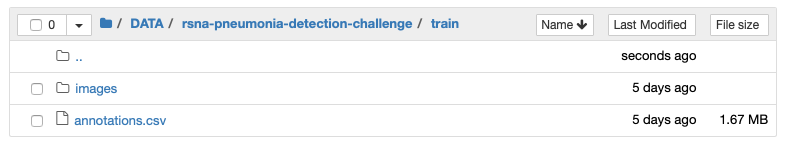
Then we created an “images” folder and extracted all images from stage_2_train_images.zip there. In the end, our dataset looked like this:

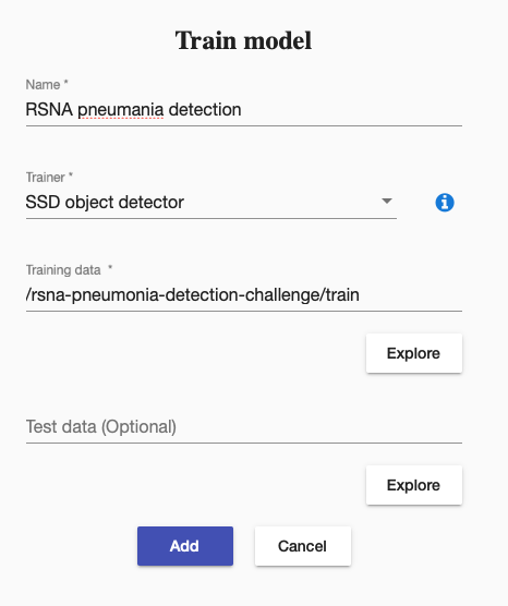
Then we created a training to train our SSD object detector. It was straightforward like this:

We started the training, it run around a day. It stoped the training by itself, when it could not increase the training accuracy any more.

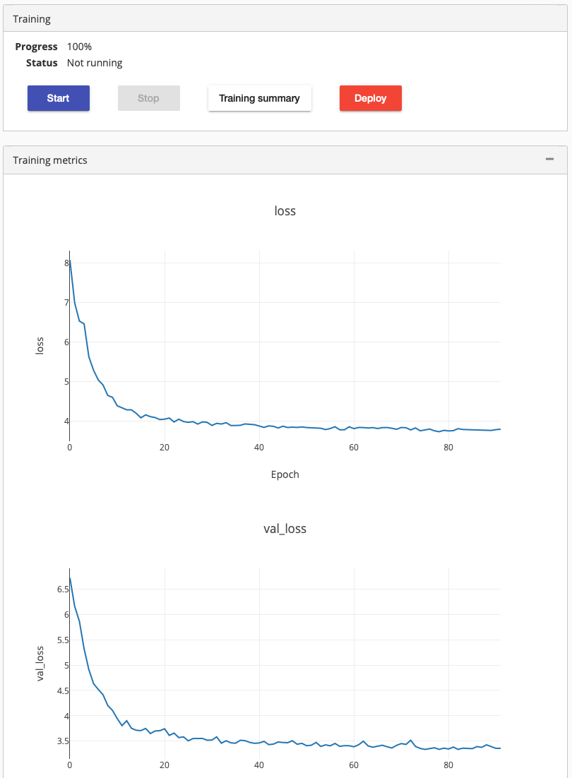
Clicking on the training summary showed mAP score 0.2725. We deployed it to check how well it performs. Testing the deployed model using a new chest radiograph gave the following result:

The prediction looks good. But how good it is, we can’t really say, since we don’t have any clinician in our team.