Analyzing breast cancer using deep learning

The process that’s used to detect breast cancer is time consuming and small malignant areas can be missed.

In order to detect cancer, a tissue section is put on a glass slide. A pathologist then examines this slide under a microscope visually scanning large regions, where there’s no cancer in order to ultimately find malignant areas. Because these glass slides can now be digitized, computer vision can be used to speed up pathologist’s workflow and provide diagnosis support.

Some terminalogy

Histopathology
This inolves examining glass tissue slides under a microscope to see if disease is present. In this case, that would be examining tissue samples from lymp nodes in order to detect breast cancer.

Whole Slide Image (WSI)
A digitized high resolution image of a glass slide taken with a scanner. The images can be several gigabytes in size. Therefore, to allow them to be used in machine learning, these digital images are cut up into patches.

Patch
A patch is a small, usually rectangular, piece of an image. For example, a 50x50 patch is a square patch containing 2500 pixels, taken from a larger image of size say 1000x1000 pixels.

Lymph Node
This is a small bean shaped structure that’s part of the body’s immune system. Lymph nodes filter substances that travel through the lymphatic fluid. They contain lymphocytes (white blood cells) that help the body fight infection and disease.

Sentinel Lymph Node
A blue dye and/or radioactive tracer is injected near the tumor. The first lymph node reached by this injected substance is called the sentinel lymph node. The images that we will be using are all of tissue samples taken from sentinel lymph nodes.

Metastasis
The spread of cancer cells to new areas of the body, often via the lymph system or bloodstream.

Data

Invasive Ductal Carcinoma (IDC) is the most common subtype of all breast cancers. Almost 80% of diagnosed breast cancers are of this subtype. This kaggle dataset consists of 277,524 patches of size 50 x 50 (198,738 IDC negative and 78,786 IDC positive), which were extracted from 162 whole mount slide images of Breast Cancer (BCa) specimens scanned at 40x. File name of each patch is of the format: u_xX_yY_classC.png (for example, 10253_idx5_x1351_y1101_class0.png), where u is the patient ID (10253_idx5), X is the x-coordinate of where this patch was cropped from, Y is the y-coordinate of where this patch was cropped from, and C indicates the class where 0 is non-IDC and 1 is IDC.

Downloading and preparing data

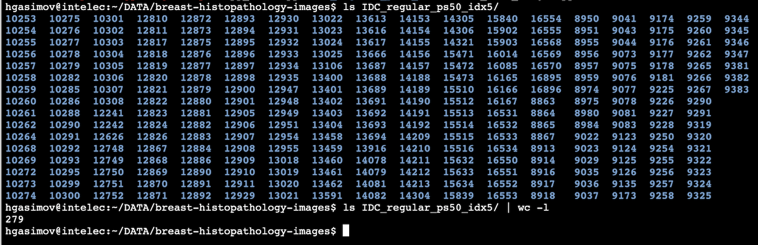
First, we need to download the dataset and unzip it. The images will be in the folder “IDC_regular_ps50_idx5”. It contains a folder for each 279 patients. Patient folders contain 2 subfolders: folder “0” with non-IDC patches and folder “1” with IDC image patches from that corresponding patient.

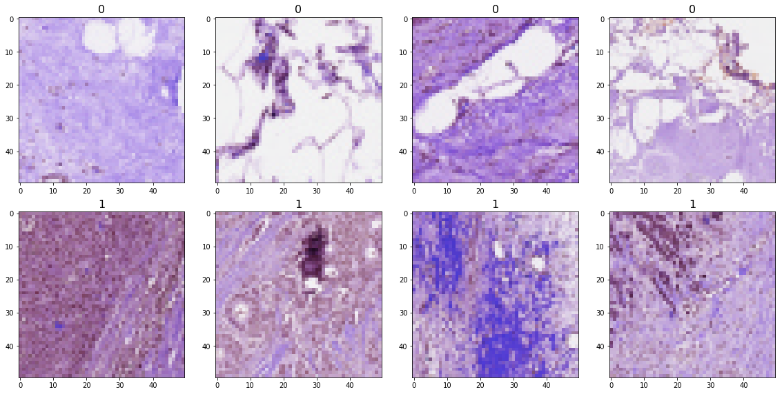
The 50x50 image pathes look like this:

Now we need to put all IDC images from all patients into one folder and all non-IDC images into another folder. One can do it manually, but we wrote a short python script to do that:

import os
from shutil import copyfile

src_folder = 'IDC_regular_ps50_idx5'
dst_folder = 'train'

os.mkdir(os.path.join(dst_folder, '0'))
os.mkdir(os.path.join(dst_folder, '1'))

folders = os.listdir(src_folder)
for f in folders:
    f_path = os.path.join(src_folder, f)
    for cl in os.listdir(f_path):
        cl_path = os.path.join(f_path, cl)
        for img in os.listdir(cl_path):
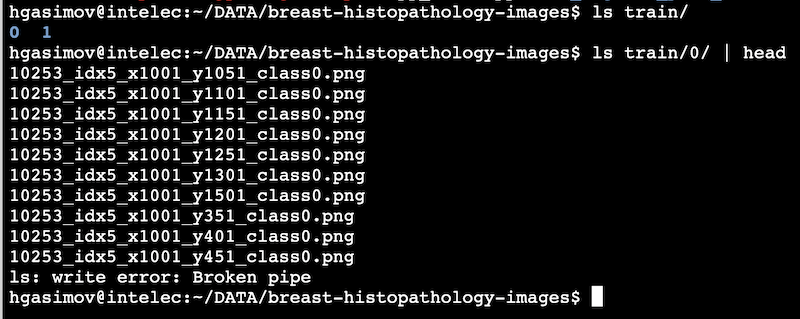
            copyfile(os.path.join(cl_path, img), os.path.join(dst_folder, cl, img))

The result will look like the following. We can use it as our training data.

Then we take 10% of training images and put into a separate folder, which we’ll use for testing. For that, we create a “test” folder and execute the following python script:

import numpy as np
import os
from shutil import move

src_folder = 'train'
dst_folder = 'test'
test_ratio = 0.1

os.mkdir(os.path.join(dst_folder, '0'))
os.mkdir(os.path.join(dst_folder, '1'))

for cl in os.listdir(src_folder):
    class_path = os.path.join(src_folder, cl)
    class_images = os.listdir(class_path)
    n_test_images = int(test_ratio*len(class_images))
    np.random.shuffle(class_images)
    for img in class_images[:n_test_images]:
        move(os.path.join(class_path, img), os.path.join(dst_folder, cl, img))

Install machine learning tools

We will use Intelec AI to create an image classifier. You can download and install it for free from here.

Training an image classifier

Intelec AI provides 2 different trainers for image classification. First one is Simple image classifier, which uses a shallow convolutional neural network (CNN). It’s pretty fast to train but the final accuracy might not be so high compared to another deeper CNNs. Second one is Deep image classifier, which takes more time to train but has better accuracy.

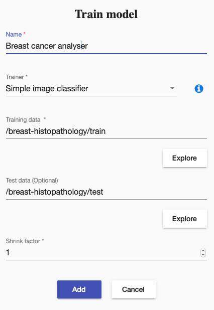
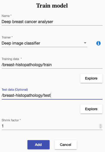
First, we created a training using Simple image classifier and started it:

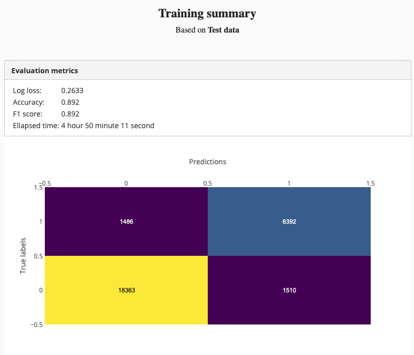
The training summary was like this:

Test set accuracy was 87%. It is not a bad result for a small model. But we can do better than that. Therefore we tried “Deep image classifier” to see, whether we can train a more accurate model.

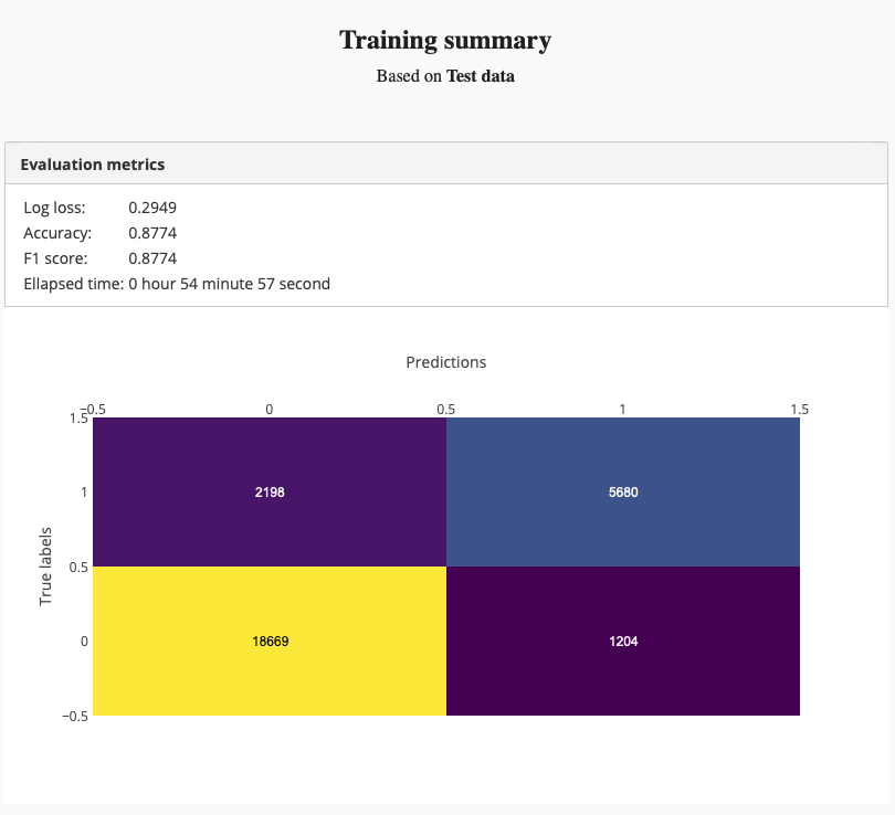
And we got better test set accuracy:

We were able able to improve the model accuracy by training a deeper network. Adding more training data might also improve the accuracy.

What experts say about computational pathology?

Prof Jeroen van der Laak, associate professor in Computational Pathology and coordinator of the highly successful CAMELYON grand challenges in 2016 and 2017, thinks computational approaches will play a major role in the future of pathology.

In the next video, features Ian Ellis, Professor of Cancer Pathology at Nottingham University, who can not imagine pathology without computational methods:

Acknowledgements

Used sources:

• Dataset from kaggle
• Kaggle kernel